0 Sionna 官方网站和文档

文章创作引用sionna官方网站及文档:

官方网站:Sionna - 6G 研究开源库 | NVIDIA 开发者 — Sionna - An Open-Source Library for 6G Research | NVIDIA Developer

官方文档:sionna文档

1 Sionna 介绍&安装

1.1 快速介绍

  • Sionna 是推进下一代通信系统(如 6G)的关键工具。
  • Sionna 基于强大的自动微分框架构建,能够通过整个通信系统反向传播梯度。这支持基于梯度的优化和机器学习,特别是神经网络集成。
  • 每个模块都是独立的,可以轻松测试、理解和根据您的需求进行修改。Sionna 提供了一个高级的 Python 应用程序编程接口(API),简化了复杂通信系统的建模。
  • Sionna 开箱即支持 NVIDIA GPU,这使得它运行速度极快。
  • Sionna 结合了信道级、链路级和系统级的仿真能力。

1.2 更多介绍

Sionna™ 是一个用于通信系统研究的硬件加速的可微分开源库。

它由
Sionna RT(用于无线电波传播建模的闪电般快速的独立式光线追踪器)
Sionna PHY(用于无线和光通信系统的链路级模拟器)
Sionna SYS(基于物理层抽象的系统级仿真功能)
三个模块组成。

Sionna PHY 和 Sionna SYS 是用 Tensorflow 编写的, Sionna RT 则基于 Mitsuba 3 和 Dr.Jit 构建。
Sionna 研究套件(RK)允许在真实的软件定义 5G NR 无线接入网络(RAN)中部署训练好的 AI/ML 组件。它基于 OpenAirInterface 项目,并由 NVIDIA Jetson AGX Orin 平台提供支持。

1.3 安装上手

说明

Sionna PHY 和 Sionna SYS 需要 Python 3.10-3.12 和 TensorFlow 2.14-2.19。
推荐使用 Ubuntu 24.04。
TensorFlow 的早期版本可能仍然可以工作,但不推荐使用。

通过pip安装(通过源代码安装方式略)

推荐通过 pip 安装 Sionna:

1
pip install sionna

如果你想在安装 Sionna 时不包含 RT 包,请运行:

1
pip install sionna-no-rt

测试、文档、开发

首先,您需要通过在仓库的根目录中执行以下命令来安装测试依赖项:

1
pip install '.[test]'

然后,你可以从 test 文件夹中运行 pytest 来执行单元测试。

通过从仓库的根目录运行以下命令来安装构建文档的要求:

1
pip install '.[doc]'

你可能需要手动安装 pandoc。然后你可以从 doc 文件夹中执行 make html 来构建文档。文档最终可以通过任何 Web 服务器来提供,例如:python -m http.server --dir build/html

开发要求可以通过从仓库的根目录执行来安装:

1
pip install '.[dev]'

通过从仓库的根目录运行 pylint src/ 可以实现代码的检查。

【略】光线追踪 Ray Tracing(RT)

2 物理层 Physical Layer(PHY)

物理层软件包提供了一个可微分的链路级模拟器。

它无缝集成了多种通信系统元素,包括前向纠错 (FEC)、多输入多输出 (MIMO) 系统、正交频分复用 (OFDM) 以及一系列无线和光信道模型。它还支持一些符合 5G NR 标准特性的模拟。

2.1 基础教程

2.1.1 sionna 入门

导入必要的库

1
2
3
4
5
6
7
8
9
10
11
12
13
14
15
16
17
18
19
20
21
22
23
24
25
26
import os # Configure which GPU
if os.getenv("CUDA_VISIBLE_DEVICES") is None:
gpu_num = 0 # Use "" to use the CPU
os.environ["CUDA_VISIBLE_DEVICES"] = f"{gpu_num}"

os.environ['TF_CPP_MIN_LOG_LEVEL'] = '3'

# Import Sionna
import sionna.phy

# Configure the notebook to use only a single GPU and allocate only as much memory as needed
# For more details, see https://www.tensorflow.org/guide/gpu
import tensorflow as tf
gpus = tf.config.list_physical_devices('GPU')
if gpus:
try:
tf.config.experimental.set_memory_growth(gpus[0], True)
except RuntimeError as e:
print(e)
# Avoid warnings from TensorFlow
tf.get_logger().setLevel('ERROR')

import numpy as np
%matplotlib inline
import matplotlib.pyplot as plt
import time

关于随机数生成的说明
固定随机种子

1
2
3
4
5
6
7
8
9
10
sionna.phy.config.seed = 40    # 修改成你的种子

# Python RNG 生成随机数
print(sionna.phy.config.py_rng.randint(0,10))

# NumPy RNG 生成随机np
print(sionna.phy.config.np_rng.integers(0,10))

# TensorFlow RNG 生成随机tf张量
print(sionna.phy.config.tf_rng.uniform(shape=[1], minval=0, maxval=10, dtype=tf.int32))

Sionna 通过批处理方式天生并行化模拟,即批处理维度中的每个元素都是独立模拟的。

tf.float32 用作首选数据类型, tf.complex64 用于复杂数值数据类型。
当需要高精度时, tf.float64 / tf.complex128 是可用的。

代码按不同任务(如信道编码、映射等)结构化为子包(详情请参阅 API 文档)。

一个简单的仿真:在 AWGN 信道上传输 QAM 符号。

首先需要创建一个 QAM 星座。

1
2
3
4
NUM_BITS_PER_SYMBOL = 2 # QPSK
constellation = sionna.phy.mapping.Constellation("qam", NUM_BITS_PER_SYMBOL)

constellation.show();

尝试更改调制阶数,例如改为 16-QAM。

然后需要设置一个映射器,将比特映射到星座点。映射器以星座作为参数。
还需要设置一个相应的解映射器,用于从接收到的含噪声样本中计算对数似然比(LLRs)。

1
2
3
4
mapper = sionna.phy.mapping.Mapper(constellation=constellation)

# The demapper uses the same constellation object as the mapper
demapper = sionna.phy.mapping.Demapper("app", constellation=constellation)

由此可见, Mapper 类继承自 Block ,即实现了一个 Sionna 块。这些块可以通过简单地将一个块的输出连接到下一个块来连接。这允许轻松构建复杂系统。

Sionna 提供了一个二进制源作为工具,用于采样均匀独立同分布的比特。
需要 AWGN 信道。

1
2
3
binary_source = sionna.phy.mapping.BinarySource()

awgn_channel = sionna.phy.channel.AWGN()

Sionna 提供了一个工具函数,用于根据比特能量与噪声功率谱密度比 $Eb/N0$  (以 dB 为单位)以及各种参数(如编码率和每符号比特数)来计算噪声功率谱密度比 $N0$ 。

1
2
3
no = sionna.phy.utils.ebnodb2no(ebno_db=10.0,
num_bits_per_symbol=NUM_BITS_PER_SYMBOL,
coderate=1.0) # Coderate set to 1 as we do uncoded transmission here

现在我们已经拥有了所有必要的组件,可以在加性高斯白噪声信道上传输 QAM 符号。Sionna 本身支持多维张量。大多数层在最后一个维度上操作,并且可以有任意的输入形状(输出时保持不变)。

1
2
3
4
5
6
7
8
9
10
11
12
13
14
BATCH_SIZE = 64 # How many examples are processed by Sionna in parallel

bits = binary_source([BATCH_SIZE,
1024]) # Blocklength
print("Shape of bits: ", bits.shape)

x = mapper(bits)
print("Shape of x: ", x.shape)

y = awgn_channel(x, no)
print("Shape of y: ", y.shape)

llr = demapper(y, no)
print("Shape of llr: ", llr.shape)
1
2
3
4
5
6
7
num_samples = 8 # how many samples shall be printed
num_symbols = int(num_samples/NUM_BITS_PER_SYMBOL)

print(f"First {num_samples} transmitted bits: {bits[0,:num_samples]}")
print(f"First {num_symbols} transmitted symbols: {np.round(x[0,:num_symbols], 2)}")
print(f"First {num_symbols} received symbols: {np.round(y[0,:num_symbols], 2)}")
print(f"First {num_samples} demapped llrs: {np.round(llr[0,:num_samples], 2)}")

可视化接收到的含噪样本。

1
2
3
4
5
6
7
8
plt.figure(figsize=(8,8))
plt.axes().set_aspect(1)
plt.grid(True)
plt.title('Channel output')
plt.xlabel('Real Part')
plt.ylabel('Imaginary Part')
plt.scatter(tf.math.real(y), tf.math.imag(y))
plt.tight_layout()

01

  • 可以通过调整信噪比来可视化对接收样本的影响。
  • 高级任务:比较“app”解映射与“maxlog”解映射的 LLR 分布。比特交织调制示例笔记本对此任务有帮助。

通信系统作为 Sionna 模块

通常更方便将基于 Sionna 的通信系统封装成一个 Sionna 模块,作为端到端模型。
这些模型可以通过堆叠不同的 Sionna 组件(即 Sionna 模块)来简单构建。

下面的单元格将之前的系统实现为一个端到端模型。

1
2
3
4
5
6
7
8
9
10
11
12
13
14
15
16
17
18
19
20
21
22
23
24
25
26
27
28
29
30
31
32
33
34
35
36
37
38
39
40
41
42
43
44
45
46
47
48
49
50
51
52
53
54
55
56
57
58
class UncodedSystemAWGN(sionna.phy.Block):
def __init__(self, num_bits_per_symbol, block_length):
"""
A Sionna Block for uncoded transmission over the AWGN channel

Parameters
----------
num_bits_per_symbol: int
The number of bits per constellation symbol, e.g., 4 for QAM16.

block_length: int
The number of bits per transmitted message block (will be the codeword length later).

Input
-----
batch_size: int
The batch_size of the Monte-Carlo simulation.

ebno_db: float
The `Eb/No` value (=rate-adjusted SNR) in dB.

Output
------
(bits, llr):
Tuple:

bits: tf.float32
A tensor of shape `[batch_size, block_length] of 0s and 1s
containing the transmitted information bits.

llr: tf.float32
A tensor of shape `[batch_size, block_length] containing the
received log-likelihood-ratio (LLR) values.
"""

super().__init__() # Must call the block initializer

self.num_bits_per_symbol = num_bits_per_symbol
self.block_length = block_length
self.constellation = sionna.phy.mapping.Constellation("qam", self.num_bits_per_symbol)
self.mapper = sionna.phy.mapping.Mapper(constellation=self.constellation)
self.demapper = sionna.phy.mapping.Demapper("app", constellation=self.constellation)
self.binary_source = sionna.phy.mapping.BinarySource()
self.awgn_channel = sionna.phy.channel.AWGN()

# @tf.function # Enable graph execution to speed things up
def call(self, batch_size, ebno_db):

# no channel coding used; we set coderate=1.0
no = sionna.phy.utils.ebnodb2no(ebno_db,
num_bits_per_symbol=self.num_bits_per_symbol,
coderate=1.0)

bits = self.binary_source([batch_size, self.block_length]) # Blocklength set to 1024 bits
x = self.mapper(bits)
y = self.awgn_channel(x, no)
llr = self.demapper(y,no)
return bits, llr

需要定义的关键函数是 __init__() ,它实例化所需的组件,以及 __call()__ ,它执行通过端到端系统的前向传递。

实例化模型:

1
model_uncoded_awgn = UncodedSystemAWGN(num_bits_per_symbol=NUM_BITS_PER_SYMBOL, block_length=1024)

Sionna 提供了一个工具,可以轻松计算和绘制误码率 (BER)。

1
2
3
4
5
6
7
8
9
10
11
12
13
EBN0_DB_MIN = -3.0 # Minimum value of Eb/N0 [dB] for simulations
EBN0_DB_MAX = 5.0 # Maximum value of Eb/N0 [dB] for simulations
BATCH_SIZE = 2000 # How many examples are processed by Sionna in parallel

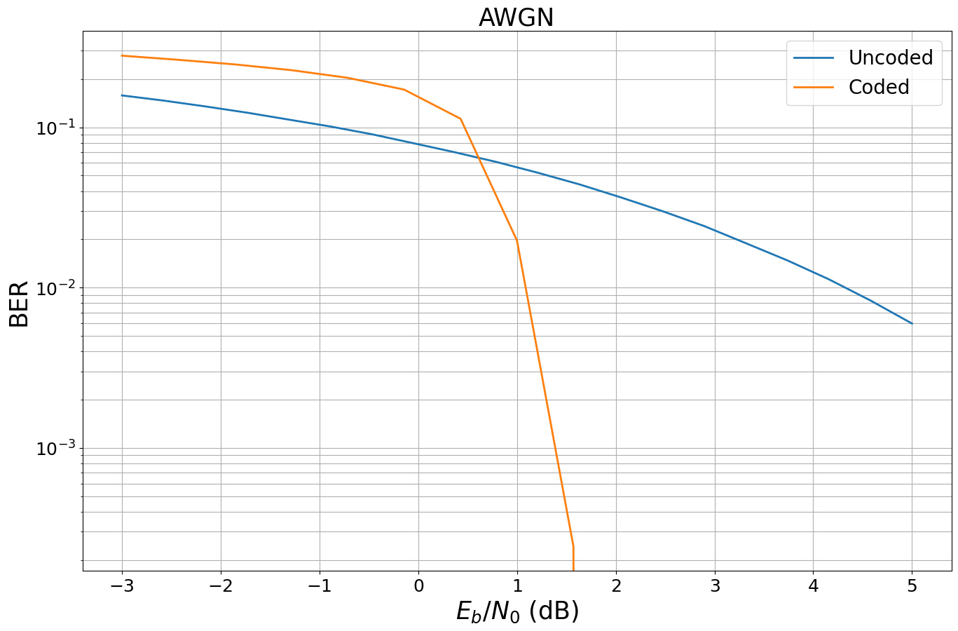
ber_plots = sionna.phy.utils.PlotBER("AWGN")
ber_plots.simulate(model_uncoded_awgn,
ebno_dbs=np.linspace(EBN0_DB_MIN, EBN0_DB_MAX, 20),
batch_size=BATCH_SIZE,
num_target_block_errors=100, # simulate until 100 block errors occured
legend="Uncoded",
soft_estimates=True,
max_mc_iter=100, # run 100 Monte-Carlo simulations (each with batch_size samples)
show_fig=True);

对象 sionna.phy.utils.PlotBER 存储结果,并允许将额外的模拟添加到先前的曲线上。

备注:在 Sionna 中,如果两个张量在最后一个维度上的至少一个位置不同(即每个码字至少有一位错误接收),则定义发生块错误。误码率是错误位置总数除以传输比特总数。

前向纠错码

我们现在向我们的收发器添加信道编码,使其更能抵抗传输错误。为此,我们将使用符合 5G 标准的低密度奇偶校验码(LDPC)码和极化码。

1
2
3
4
5
k = 12
n = 20

encoder = sionna.phy.fec.ldpc.LDPC5GEncoder(k, n)
decoder = sionna.phy.fec.ldpc.LDPC5GDecoder(encoder, hard_out=True)

对一些随机输入比特进行编码:

1
2
3
4
5
6
BATCH_SIZE = 1 # one codeword in parallel
u = binary_source([BATCH_SIZE, k])
print("Input bits are: \n", u.numpy())

c = encoder(u)
print("Encoded bits are: \n", c.numpy())

Sionna 的一个基本范式是批量处理。因此,上述示例可以针对任意批处理大小来并行模拟 batch_size 编码字。

🚨 重点!

1
2
3
4
5
6
7
8
9
10
11
12
13
14
15
16
17
18
19
20
21
22
23
24
25
26
27
28
29
30
然而,Sionna 的功能更多——它支持 N 维输入张量,从而允许在单个命令行中处理多个用户和多个天线的多个样本。假设我们想要为每个连接到每个的 `num_users` 个用户编码长度为 `n` 的 `batch_size` 个码字。这意味着总共传输 `batch_size` * `n` * `num_users` * `num_basestations` 个比特。
```python
BATCH_SIZE = 10 # samples per scenario
num_basestations = 4
num_users = 5 # users per basestation
n = 1000 # codeword length per transmitted codeword
coderate = 0.5 # coderate

k = int(coderate * n) # number of info bits per codeword

# instantiate a new encoder for codewords of length n
encoder = sionna.phy.fec.ldpc.LDPC5GEncoder(k, n)

# the decoder must be linked to the encoder (to know the exact code parameters used for encoding)
decoder = sionna.phy.fec.ldpc.LDPC5GDecoder(encoder,
hard_out=True, # binary output or provide soft-estimates
return_infobits=True, # or also return (decoded) parity bits
num_iter=20, # number of decoding iterations
cn_update="boxplus-phi") # also try "minsum" decoding

# draw random bits to encode
u = binary_source([BATCH_SIZE, num_basestations, num_users, k])
print("Shape of u: ", u.shape)

# We can immediately encode u for all users, basetation and samples
# This all happens with a single line of code
c = encoder(u)
print("Shape of c: ", c.shape)

print("Total number of processed bits: ", np.prod(c.shape))

这种方式适用于任意维度,并允许将设计的系统简单地扩展到多用户或多天线场景。

用极码替换 LDPC 码。API 保持相似。

1
2
3
4
5
6
k = 64
n = 128

encoder = sionna.phy.fec.polar.Polar5GEncoder(k, n)
decoder = sionna.phy.fec.polar.Polar5GDecoder(encoder,
dec_type="SCL") # you can also use "SCL"

高级备注:5G 极码编解码器类直接应用速率匹配和额外的 CRC 级联。所有这些操作都在内部完成,对用户透明。如果您想访问极码的低级功能,请使用 sionna.fec.polar.PolarEncoder 和所需的解码器( sionna.fec.polar.PolarSCDecoder 、 sionna.fec.polar.PolarSCLDecoder 或 sionna.fec.polar.PolarBPDecoder )。

更多细节可以在 5G 信道编码和速率匹配的教程笔记本中找到: 5G 极化码与 LDPC 码的比较
02

将带编码的模块封装成通信系统

1
2
3
4
5
6
7
8
9
10
11
12
13
14
15
16
17
18
19
20
21
22
23
24
25
26
27
28
29
30
class CodedSystemAWGN(sionna.phy.Block):
def __init__(self, num_bits_per_symbol, n, coderate):
super().__init__() # Must call the Sionna block initializer

self.num_bits_per_symbol = num_bits_per_symbol
self.n = n
self.k = int(n*coderate)
self.coderate = coderate
self.constellation = sionna.phy.mapping.Constellation("qam", self.num_bits_per_symbol)

self.mapper = sionna.phy.mapping.Mapper(constellation=self.constellation)
self.demapper = sionna.phy.mapping.Demapper("app", constellation=self.constellation)

self.binary_source = sionna.phy.mapping.BinarySource()
self.awgn_channel = sionna.phy.channel.AWGN()

self.encoder = sionna.phy.fec.ldpc.LDPC5GEncoder(self.k, self.n)
self.decoder = sionna.phy.fec.ldpc.LDPC5GDecoder(self.encoder, hard_out=True)

#@tf.function # activate graph execution to speed things up
def call(self, batch_size, ebno_db):
no = sionna.phy.utils.ebnodb2no(ebno_db, num_bits_per_symbol=self.num_bits_per_symbol, coderate=self.coderate)

bits = self.binary_source([batch_size, self.k])
codewords = self.encoder(bits)
x = self.mapper(codewords)
y = self.awgn_channel(x, no)
llr = self.demapper(y,no)
bits_hat = self.decoder(llr)
return bits, bits_hat

仿真:

1
2
3
4
5
6
7
8
9
10
11
12
13
14
15
CODERATE = 0.5
BATCH_SIZE = 2000

model_coded_awgn = CodedSystemAWGN(num_bits_per_symbol=NUM_BITS_PER_SYMBOL,
n=2048,
coderate=CODERATE)
ber_plots.simulate(model_coded_awgn,
ebno_dbs=np.linspace(EBN0_DB_MIN, EBN0_DB_MAX, 15),
batch_size=BATCH_SIZE,
num_target_block_errors=500,
legend="Coded",
soft_estimates=False,
max_mc_iter=15,
show_fig=True,
forward_keyboard_interrupt=False);

03

急切Eager模式和图Graph模式

以上内容以 eager 模式执行了示例。这允许像编写 NumPy 一样运行 TensorFlow 操作,简化了开发和调试。
然而,为了发挥 Sionna 的全部性能,我们需要激活 graph 模式,这可以通过函数装饰器 @tf.function() 来启用。

1
2
3
4
5
6
7
8
9
10
11
12
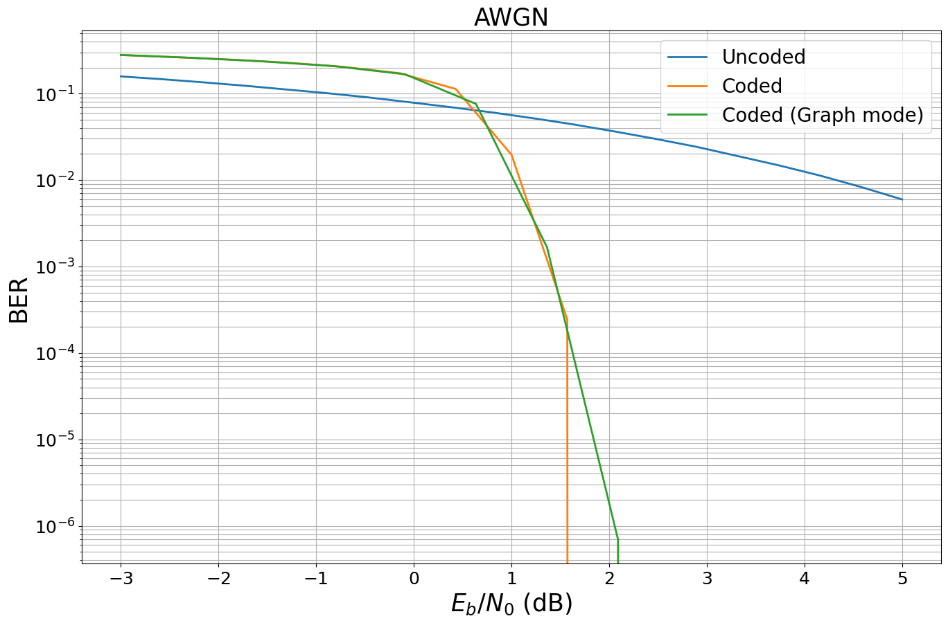
@tf.function() # enables graph-mode of the following function
def run_graph(batch_size, ebno_db):
# all code inside this function will be executed in graph mode, also calls of other functions
print(f"Tracing run_graph for values batch_size={batch_size} and ebno_db={ebno_db}.") # print whenever this function is traced
return model_coded_awgn(batch_size, ebno_db)


batch_size = 10 # try also different batch sizes
ebno_db = 1.5

# run twice - how does the output change?
run_graph(batch_size, ebno_db)

在图模式下,Python 代码(即非 TensorFlow 代码)仅在函数被跟踪时执行。这发生在输入签名发生变化时。

为了避免针对不同输入的重新追踪,我们现在输入张量。你可以看到,现在对于相同数据类型的输入张量,函数只被追踪一次。

注意:如果函数的输入是一个张量,其签名必须改变而不仅仅是值。例如,输入的大小或数据类型可能不同。为了高效地执行代码,我们通常希望在不需要的情况下避免重新追踪代码。

以图形模式运行与上述相同的模拟。

1
2
3
4
5
6
7
8
9
10
11
12
13
14
15
16
17
18
19
20
21
22
23
24
25
26
27
28
repetitions = 4 # average over multiple runs
batch_size = BATCH_SIZE # try also different batch sizes
ebno_db = 1.5

# --- eager mode ---
t_start = time.perf_counter()
for _ in range(repetitions):
bits, bits_hat = model_coded_awgn(tf.constant(batch_size, tf.int32),
tf.constant(ebno_db, tf. float32))
t_stop = time.perf_counter()
# throughput in bit/s
throughput_eager = np.size(bits.numpy())*repetitions / (t_stop - t_start) / 1e6

print(f"Throughput in Eager mode: {throughput_eager :.3f} Mbit/s")
# --- graph mode ---
# run once to trace graph (ignored for throughput)
run_graph(tf.constant(batch_size, tf.int32),
tf.constant(ebno_db, tf. float32))

t_start = time.perf_counter()
for _ in range(repetitions):
bits, bits_hat = run_graph(tf.constant(batch_size, tf.int32),
tf.constant(ebno_db, tf. float32))
t_stop = time.perf_counter()
# throughput in bit/s
throughput_graph = np.size(bits.numpy())*repetitions / (t_stop - t_start) / 1e6

print(f"Throughput in graph mode: {throughput_graph :.3f} Mbit/s")
1
2
3
4
5
6
7
8
9
ber_plots.simulate(run_graph,
ebno_dbs=np.linspace(EBN0_DB_MIN, EBN0_DB_MAX, 12),
batch_size=BATCH_SIZE,
num_target_block_errors=500,
legend="Coded (Graph mode)",
soft_estimates=True,
max_mc_iter=100,
show_fig=True,
forward_keyboard_interrupt=False);

04

1

2.2 进阶教程